The gapminder object contains structured data in the form of a data frame, which organizes data into rows and columns akin to a spreadsheet or a SQL database table. Data analyses in R, including those in this course, predominantly revolve around data frames. While the gapminder data is presented as a special type of data frame known as a tibble, the distinction is not crucial at this point.
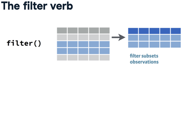
R initially displays the first ten rows of the data frame, offering a glimpse of its contents along with a brief description. This description indicates that the tibble comprises 1,704 rows, referred to as observations, and six columns, termed variables. Understanding the meaning of each observation, or row, is pivotal in analysis. In this dataset, each observation signifies a unique combination of country and year. For instance, the first observation pertains to Afghanistan’s statistics in 1952, followed by subsequent observations for the same country in different years.
For every country-year combination, the dataset provides several variables detailing the country’s demographics. These variables include the continent (e.g., Asia), life expectancy, population, and GDP per capita. GDP per capita denotes a country’s total economic output (Gross Domestic Product) divided by its population, serving as a common metric for assessing a country’s wealth. Each variable adheres to a consistent data type: numeric for measures like life expectancy and population, and categorical for attributes like country and continent.
Even from this limited view of the data, one can glean insights. For instance, examining Afghanistan’s data reveals an increase in both life expectancy and population over time, while GDP per capita fluctuates. Throughout the course, you’ll learn how to leverage R to draw numerous conclusions about the social and economic histories of countries worldwide.