Project: Sowing Success - How Machine Learning Helps Farmers Select the Best Crops

Measuring essential soil metrics such as nitrogen, phosphorous, potassium levels, and pH value is an important aspect of assessing soil condition. However, it can be an expensive and time-consuming process, which can cause farmers to prioritize which metrics to measure based on their budget constraints.
Farmers have various options when it comes to deciding which crop to plant each season. Their primary objective is to maximize the yield of their crops, taking into account different factors. One crucial factor that affects crop growth is the condition of the soil in the field, which can be assessed by measuring basic elements such as nitrogen and potassium levels. Each crop has an ideal soil condition that ensures optimal growth and maximum yield.
A farmer reached out to you as a machine learning expert for assistance in selecting the best crop for his field. They’ve provided you with a dataset called soil_measures.csv, which contains:
"N": Nitrogen content ratio in the soil"P": Phosphorous content ratio in the soil"K": Potassium content ratio in the soil"pH"value of the soil"crop": categorical values that contain various crops (target variable).
Each row in this dataset represents various measures of the soil in a particular field. Based on these measurements, the crop specified in the "crop" column is the optimal choice for that field.
In this project, you will apply machine learning to build a multi-class classification model to predict the type of "crop", while using techniques to avoid multicollinearity, which is a concept where two or more features are highly correlated.
Instructions
Build a multi-class Logistic Regression model to predict categories of “crop” with a F1 score of more than 0.5.
Read in soil_measures.csv as a pandas DataFrame and perform some data checks, such as determining the number of crops, checking for missing values, and verifying that the data in each potential feature column is numeric.
Split the data into training and test sets, setting test_size equal to 20% and using a random_state of 42.
Predict the “crop” type using each feature individually by looping over all the features, and, for each feature, fit a Logistic Regression model and calculate f1_score(). When creating the model, set max_iter to 2000 so the model can converge, and pass an appropriate string value to the multi_class keyword argument.
In order to avoid selecting two features that are highly correlated, perform a correlation analysis for each pair of features, enabling you to build a final model without the presence of multicollinearity.
Once you have your final features, train and test a new Logistic Regression model called log_reg, then evaluate performance using f1_score(), saving the metric as a variable called model_performance.
# All required libraries are imported here for you.
import matplotlib.pyplot as plt
import pandas as pd
from sklearn.linear_model import LogisticRegression
from sklearn.model_selection import train_test_split
import seaborn as sns
from sklearn.metrics import f1_score

# Load the dataset
crops = pd.read_csv("datasets/soil_measures.csv")

# Write your code here
#Individual crops
crop=crops['crop'].unique()
print(len(crop))22Split the data into training and test sets, setting test_size equal to 20% and using a random_state of 42.
y = crops['crop']
X = crops.drop("crop", axis=1)

X_train, X_test, y_train, y_test = train_test_split(X, y, test_size=0.2, random_state=42)
Predict the “crop” type using each feature individually by looping over all the features, and, for each feature, fit a Logistic Regression model and calculate f1_score(). When creating the model, set max_iter to 2000 so the model can converge, and pass an appropriate string value to the multi_class keyword argument.
from sklearn.model_selection import train_test_split
from sklearn.linear_model import LogisticRegression
from sklearn.metrics import f1_score

logreg = LogisticRegression(multi_class='multinomial', max_iter=2000)
for c in X_train.columns:
    dt_train = X_train[[c]]  # Selecting the current feature for training
    dt_test = X_test[[c]]    # Selecting the current feature for testing

    logreg.fit(dt_train, y_train)
    y_pred = logreg.predict(dt_test)

    f1 = f1_score(y_test, y_pred, average='weighted')
    print(f"F1 score using feature '{c}': {f1}")
F1 score using feature 'N': 0.10507916708090527
F1 score using feature 'P': 0.10457380486654515
F1 score using feature 'K': 0.2007873036107074
F1 score using feature 'ph': 0.04532731061152114In order to avoid selecting two features that are highly correlated, perform a correlation analysis for each pair of features, enabling you to build a final model without the presence of multicollinearity.
import seaborn as sns
import matplotlib.pyplot as plt

# Calculate the correlation matrix
correlation_matrix = X.corr()

# Plotting the correlation heatmap
plt.figure(figsize=(8, 6))
sns.heatmap(correlation_matrix, annot=True, cmap='coolwarm', fmt=".2f")
plt.title('Correlation Heatmap of Features')
plt.show()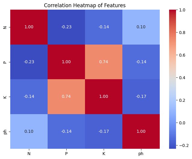
Feature ‘K’ and ‘P’ are highly co-related. Dropping ‘P’
final_features = ['N', 'K', 'ph']X = X[final_features]
X_train, X_test, y_train, y_test = train_test_split(X, y, test_size=0.2, random_state=42)from sklearn.model_selection import train_test_split
from sklearn.linear_model import LogisticRegression
from sklearn.metrics import f1_score
log_reg = LogisticRegression(multi_class='multinomial', max_iter=2000)
log_reg.fit(X_train, y_train)
y_pred = log_reg.predict(X_test)
model_performance = f1_score(y_test, y_pred, average='weighted')model_performance0.558010495235685