Joining Data with pandas
# Import pandas
import pandas as pd

# Import some of the course datasets
actors_movies = pd.read_csv("datasets/actors_movies.csv")
business_owners = pd.read_pickle("datasets/business_owners.p")
casts = pd.read_pickle("datasets/casts.p")

# Preview one of the DataFrames
casts
Chapter 1: Data Merging Basics
Learn how you can merge disparate data using inner joins. By combining information from multiple sources you’ll uncover compelling insights that may have previously been hidden. You’ll also learn how the relationship between those sources, such as one-to-one or one-to-many, can affect your result.
Your first inner join
You have been tasked with figuring out what the most popular types of fuel used in Chicago taxis are. To complete the analysis, you need to merge the taxi_owners and taxi_veh tables together on the vid column. You can then use the merged table along with the .value_counts() method to find the most common fuel_type.
Since you’ll be working with pandas throughout the course, the package will be preloaded for you as pd in each exercise in this course. Also the taxi_owners and taxi_veh DataFrames are loaded for you. ### Instructions - Merge taxi_owners with taxi_veh on the column vid, and save the result to taxi_own_veh. - Set the left and right table suffixes for overlapping columns of the merge to _own and _veh, respectively. - Select the fuel_type column from taxi_own_veh and print the value_counts() to find the most popular fuel_types used.
taxi_owners = pd.read_pickle("datasets/taxi_owners.p")
taxi_veh = pd.read_pickle("datasets/taxi_vehicles.p")
print(taxi_owners.head(3))
print(taxi_veh.head(3))
rid vid owner address zip
0 T6285 6285 AGEAN TAXI LLC 4536 N. ELSTON AVE. 60630
1 T4862 4862 MANGIB CORP. 5717 N. WASHTENAW AVE. 60659
2 T1495 1495 FUNRIDE, INC. 3351 W. ADDISON ST. 60618
vid make model year fuel_type owner
0 2767 TOYOTA CAMRY 2013 HYBRID SEYED M. BADRI
1 1411 TOYOTA RAV4 2017 HYBRID DESZY CORP.
2 6500 NISSAN SENTRA 2019 GASOLINE AGAPH CAB CORP
# Merge the taxi_owners and taxi_veh tables
taxi_own_veh = taxi_owners.merge(taxi_veh, on = 'vid')

# Print the column names of the taxi_own_veh
print(taxi_own_veh.columns)
Index(['rid', 'vid', 'owner_x', 'address', 'zip', 'make', 'model', 'year',
'fuel_type', 'owner_y'],
dtype='object')# Merge the taxi_owners and taxi_veh tables setting a suffix
taxi_own_veh = taxi_owners.merge(taxi_veh, on='vid', suffixes = ("_own","_veh"))
# Print the column names of taxi_own_veh
print(taxi_own_veh.columns)Index(['rid', 'vid', 'owner_own', 'address', 'zip', 'make', 'model', 'year',
'fuel_type', 'owner_veh'],
dtype='object')# Merge the taxi_owners and taxi_veh tables setting a suffix
taxi_own_veh = taxi_owners.merge(taxi_veh, on='vid', suffixes=('_own','_veh'))
# Print the value_counts to find the most popular fuel_type
print(taxi_own_veh['fuel_type'].value_counts())HYBRID 2792
GASOLINE 611
FLEX FUEL 89
COMPRESSED NATURAL GAS 27
Name: fuel_type, dtype: int64Inner joins and number of rows returned
All of the merges you have studied to this point are called inner joins. It is necessary to understand that inner joins only return the rows with matching values in both tables. You will explore this further by reviewing the merge between the wards and census tables, then comparing it to merges of copies of these tables that are slightly altered, named wards_altered, and census_altered. The first row of the wards column has been changed in the altered tables. You will examine how this affects the merge between them. The tables have been loaded for you.
For this exercise, it is important to know that the wards and census tables start with 50 rows. ### Instructions - Merge wards and census on the ward column and save the result to wards_census. - Merge the wards_altered and census tables on the ward column, and notice the difference in returned rows. - Merge the wards and census_altered tables on the ward column, and notice the difference in returned rows.
wards = pd.read_pickle("datasets/ward.p")
print(wards.head(3))

census = pd.read_pickle("datasets/census.p")
print(census.head(3))
ward alderman address zip
0 1 Proco "Joe" Moreno 2058 NORTH WESTERN AVENUE 60647
1 2 Brian Hopkins 1400 NORTH ASHLAND AVENUE 60622
2 3 Pat Dowell 5046 SOUTH STATE STREET 60609
ward pop_2000 pop_2010 change address zip
0 1 52951 56149 6% 2765 WEST SAINT MARY STREET 60647
1 2 54361 55805 3% WM WASTE MANAGEMENT 1500 60622
2 3 40385 53039 31% 17 EAST 38TH STREET 60653# Merge the wards and census tables on the ward column
wards_census = wards.merge(census, on ='ward')
# Print the shape of wards_census
print('wards_census table shape:', wards_census.shape)wards_census table shape: (50, 9)# Print the first few rows of the wards_altered table to view the change
print(wards_altered[['ward']].head())
# Merge the wards_altered and census tables on the ward column
wards_altered_census = wards_altered.merge(census, on = 'ward')
# Print the shape of wards_altered_census
print('wards_altered_census table shape:', wards_altered_census.shape)One-to-many merge
A business may have one or multiple owners. In this exercise, you will continue to gain experience with one-to-many merges by merging a table of business owners, called biz_owners, to the licenses table. Recall from the video lesson, with a one-to-many relationship, a row in the left table may be repeated if it is related to multiple rows in the right table. In this lesson, you will explore this further by finding out what is the most common business owner title. (i.e., secretary, CEO, or vice president)
The licenses and biz_owners DataFrames are loaded for you. ### Instructions - Starting with the licenses table on the left, merge it to the biz_owners table on the column account, and save the results to a variable named licenses_owners. - Group licenses_owners by title and count the number of accounts for each title. Save the result as counted_df - Sort counted_df by the number of accounts in descending order, and save this as a variable named sorted_df. - Use the .head() method to print the first few rows of the sorted_df.
licenses = pd.read_pickle("datasets/licenses.p")
print(licenses.head(3))
biz_owners = pd.read_pickle("datasets/business_owners.p")
print(biz_owners.head(3))
account ward aid business address zip
0 307071 3 743 REGGIE'S BAR & GRILL 2105 S STATE ST 60616
1 10 10 829 HONEYBEERS 13200 S HOUSTON AVE 60633
2 10002 14 775 CELINA DELI 5089 S ARCHER AVE 60632
account first_name last_name title
0 10 PEARL SHERMAN PRESIDENT
1 10 PEARL SHERMAN SECRETARY
2 10002 WALTER MROZEK PARTNER# Merge the licenses and biz_owners table on account
licenses_owners = licenses.merge(biz_owners, on = 'account')
# Group the results by title then count the number of accounts
counted_df = licenses_owners.groupby('title').agg({'account':'count'})
# Sort the counted_df in desending order
sorted_df = counted_df.sort_values(by = 'account',ascending=False)
# Use .head() method to print the first few rows of sorted_df
print(sorted_df.head()) account
title
PRESIDENT 6259
SECRETARY 5205
SOLE PROPRIETOR 1658
OTHER 1200
VICE PRESIDENT 970Total riders in a month
Your goal is to find the total number of rides provided to passengers passing through the Wilson station (station_name == ‘Wilson’) when riding Chicago’s public transportation system on weekdays (day_type == ‘Weekday’) in July (month == 7). Luckily, Chicago provides this detailed data, but it is in three different tables. You will work on merging these tables together to answer the question. This data is different from the business related data you have seen so far, but all the information you need to answer the question is provided.
Instructions
- Merge the ridership and cal tables together, starting with the ridership table on the left and save the result to the variable ridership_cal. If you code takes too long to run, your merge conditions might be incorrect.
- Extend the previous merge to three tables by also merging the stations table.
- Create a variable called filter_criteria to select the appropriate rows from the merged table so that you can sum the rides column.
ridership = pd.read_pickle("datasets/cta_ridership.p")
ridership.head(3)| station_id | year | month | day | rides | |
|---|---|---|---|---|---|
| 0 | 40010 | 2019 | 1 | 1 | 576 |
| 1 | 40010 | 2019 | 1 | 2 | 1457 |
| 2 | 40010 | 2019 | 1 | 3 | 1543 |
stations = pd.read_pickle("datasets/stations.p")
stations.head(4)| station_id | station_name | location | |
|---|---|---|---|
| 0 | 40010 | Austin-Forest Park | (41.870851, -87.776812) |
| 1 | 40020 | Harlem-Lake | (41.886848, -87.803176) |
| 2 | 40030 | Pulaski-Lake | (41.885412, -87.725404) |
| 3 | 40040 | Quincy/Wells | (41.878723, -87.63374) |
cal = pd.read_pickle("datasets/cta_calendar.p")
cal.head(4)| year | month | day | day_type | |
|---|---|---|---|---|
| 0 | 2019 | 1 | 1 | Sunday/Holiday |
| 1 | 2019 | 1 | 2 | Weekday |
| 2 | 2019 | 1 | 3 | Weekday |
| 3 | 2019 | 1 | 4 | Weekday |
# Merge the ridership and cal tables
ridership_cal = ridership.merge(cal)
# Merge the ridership, cal, and stations tables
ridership_cal_stations = ridership.merge(cal, on=['year','month','day']) \
.merge(stations,on="station_id")# Merge the ridership, cal, and stations tables
ridership_cal_stations = ridership.merge(cal, on=['year','month','day']) \
.merge(stations, on='station_id')
# Create a filter to filter ridership_cal_stations
filter_criteria = ((ridership_cal_stations['month'] == 7)
& (ridership_cal_stations['day_type'] == 'Weekday')
& (ridership_cal_stations['station_name'] == 'Wilson'))
# Use .loc and the filter to select for rides
print(ridership_cal_stations.loc[filter_criteria, 'rides'].sum())140005Three table merge
To solidify the concept of a three DataFrame merge, practice another exercise. A reasonable extension of our review of Chicago business data would include looking at demographics information about the neighborhoods where the businesses are. A table with the median income by zip code has been provided to you. You will merge the licenses and wards tables with this new income-by-zip-code table called zip_demo.
The licenses, wards, and zip_demo DataFrames have been loaded for you. ### Instructions - Starting with the licenses table, merge to it the zip_demo table on the zip column. Then merge the resulting table to the wards table on the ward column. Save result of the three merged tables to a variable named licenses_zip_ward. - Group the results of the three merged tables by the column alderman and find the median income.
zip_demo = pd.read_pickle("datasets/zip_demo.p")
zip_demo.head(4)| zip | income | |
|---|---|---|
| 0 | 60630 | 70122 |
| 1 | 60640 | 50488 |
| 2 | 60622 | 87143 |
| 3 | 60614 | 100116 |
# Merge licenses and zip_demo, on zip; and merge the wards on ward
licenses_zip_ward = licenses.merge(zip_demo, on ="zip") \
                        .merge(wards, on = "ward")

# Print the results by alderman and show median income
print(licenses_zip_ward.groupby("alderman").agg({'income':'median'}))
income
alderman
Ameya Pawar 66246.0
Anthony A. Beale 38206.0
Anthony V. Napolitano 82226.0
Ariel E. Reyboras 41307.0
Brendan Reilly 110215.0
Brian Hopkins 87143.0
Carlos Ramirez-Rosa 66246.0
Carrie M. Austin 38206.0
Chris Taliaferro 55566.0
Daniel "Danny" Solis 41226.0
David H. Moore 33304.0
Deborah Mell 66246.0
Debra L. Silverstein 50554.0
Derrick G. Curtis 65770.0
Edward M. Burke 42335.0
Emma M. Mitts 36283.0
George Cardenas 33959.0
Gilbert Villegas 41307.0
Gregory I. Mitchell 24941.0
Harry Osterman 45442.0
Howard B. Brookins, Jr. 33304.0
James Cappleman 79565.0
Jason C. Ervin 41226.0
Joe Moore 39163.0
John S. Arena 70122.0
Leslie A. Hairston 28024.0
Margaret Laurino 70122.0
Marty Quinn 67045.0
Matthew J. O'Shea 59488.0
Michael R. Zalewski 42335.0
Michael Scott, Jr. 31445.0
Michelle A. Harris 32558.0
Michelle Smith 100116.0
Milagros "Milly" Santiago 41307.0
Nicholas Sposato 62223.0
Pat Dowell 46340.0
Patrick Daley Thompson 41226.0
Patrick J. O'Connor 50554.0
Proco "Joe" Moreno 87143.0
Raymond A. Lopez 33959.0
Ricardo Munoz 31445.0
Roberto Maldonado 68223.0
Roderick T. Sawyer 32558.0
Scott Waguespack 68223.0
Susan Sadlowski Garza 38417.0
Tom Tunney 88708.0
Toni L. Foulkes 27573.0
Walter Burnett, Jr. 87143.0
William D. Burns 107811.0
Willie B. Cochran 28024.0One-to-many merge with multiple tables
In this exercise, assume that you are looking to start a business in the city of Chicago. Your perfect idea is to start a company that uses goats to mow the lawn for other businesses. However, you have to choose a location in the city to put your goat farm. You need a location with a great deal of space and relatively few businesses and people around to avoid complaints about the smell. You will need to merge three tables to help you choose your location. The land_use table has info on the percentage of vacant land by city ward. The census table has population by ward, and the licenses table lists businesses by ward.
The land_use, census, and licenses tables have been loaded for you. ### Instructions - Merge land_use and census on the ward column. Merge the result of this with licenses on the ward column, using the suffix _cen for the left table and _lic for the right table. Save this to the variable land_cen_lic. - Group land_cen_lic by ward, pop_2010 (the population in 2010), and vacant, then count the number of accounts. Save the results to pop_vac_lic. - Sort pop_vac_lic by vacant, account, andpop_2010 in descending, ascending, and ascending order respectively. Save it as sorted_pop_vac_lic.
land_use = pd.read_pickle("datasets/land_use.p")
land_use.head(4)| ward | residential | commercial | industrial | vacant | other | |
|---|---|---|---|---|---|---|
| 0 | 1 | 41 | 9 | 2 | 2 | 46 |
| 1 | 2 | 31 | 11 | 6 | 2 | 50 |
| 2 | 3 | 20 | 5 | 3 | 13 | 59 |
| 3 | 4 | 22 | 13 | 0 | 7 | 58 |
# Merge land_use and census and merge result with licenses including suffixes
land_cen_lic = land_use.merge(census, on = "ward").merge(licenses, on = "ward", suffixes = ("_cen","_lic"))
# Merge land_use and census and merge result with licenses including suffixes
land_cen_lic = land_use.merge(census, on='ward') \
.merge(licenses, on='ward', suffixes=('_cen','_lic'))
# Group by ward, pop_2010, and vacant, then count the # of accounts
pop_vac_lic = land_cen_lic.groupby(['ward',"pop_2010","vacant"],
as_index=False).agg({'account':'count'})# Merge land_use and census and merge result with licenses including suffixes
land_cen_lic = land_use.merge(census, on='ward') \
.merge(licenses, on='ward', suffixes=('_cen','_lic'))
# Group by ward, pop_2010, and vacant, then count the # of accounts
pop_vac_lic = land_cen_lic.groupby(['ward','pop_2010','vacant'],
as_index=False).agg({'account':'count'})
# Sort pop_vac_lic and print the results
sorted_pop_vac_lic = pop_vac_lic.sort_values(by = ["vacant","account","pop_2010"],
ascending=[False,True,True])
# Print the top few rows of sorted_pop_vac_lic
print(sorted_pop_vac_lic.head()) ward pop_2010 vacant account
47 7 51581 19 80
12 20 52372 15 123
1 10 51535 14 130
16 24 54909 13 98
7 16 51954 13 156Chapter 2: Merging Tables With Different Join Types
Take your knowledge of joins to the next level. In this chapter, you’ll work with TMDb movie data as you learn about left, right, and outer joins. You’ll also discover how to merge a table to itself and merge on a DataFrame index.
Enriching a dataset
Setting how=‘left’ with the .merge()method is a useful technique for enriching or enhancing a dataset with additional information from a different table. In this exercise, you will start off with a sample of movie data from the movie series Toy Story. Your goal is to enrich this data by adding the marketing tag line for each movie. You will compare the results of a left join versus an inner join.
The toy_story DataFrame contains the Toy Story movies. The toy_story and taglines DataFrames have been loaded for you. ### Instructions - Merge toy_story and taglines on the id column with a left join, and save the result as toystory_tag. - With toy_story as the left table, merge to it taglines on the id column with an inner join, and save as toystory_tag.
movies = pd.read_pickle("datasets/movies.p")
movies.head(4)
toy_story = movies[movies["title"].str.contains("Toy Story")].reset_index(drop=True)
toy_story| id | title | popularity | release_date | |
|---|---|---|---|---|
| 0 | 10193 | Toy Story 3 | 59.995418 | 2010-06-16 |
| 1 | 863 | Toy Story 2 | 73.575118 | 1999-10-30 |
| 2 | 862 | Toy Story | 73.640445 | 1995-10-30 |
taglines = pd.read_pickle("datasets/taglines.p")
taglines.head(4)| id | tagline | |
|---|---|---|
| 0 | 19995 | Enter the World of Pandora. |
| 1 | 285 | At the end of the world, the adventure begins. |
| 2 | 206647 | A Plan No One Escapes |
| 3 | 49026 | The Legend Ends |
# Merge the toy_story and taglines tables with a left join
toystory_tag = toy_story.merge(taglines, how = "left", on="id")

# Print the rows and shape of toystory_tag
print(toystory_tag)
print(toystory_tag.shape)
id title popularity release_date tagline
0 10193 Toy Story 3 59.995418 2010-06-16 No toy gets left behind.
1 863 Toy Story 2 73.575118 1999-10-30 The toys are back!
2 862 Toy Story 73.640445 1995-10-30 NaN
(3, 5)# Merge the toy_story and taglines tables with a inner join
toystory_tag = toy_story.merge(taglines,on="id")
# Print the rows and shape of toystory_tag
print(toystory_tag)
print(toystory_tag.shape) id title popularity release_date tagline
0 10193 Toy Story 3 59.995418 2010-06-16 No toy gets left behind.
1 863 Toy Story 2 73.575118 1999-10-30 The toys are back!
(2, 5)Right join to find unique movies
Most of the recent big-budget science fiction movies can also be classified as action movies. You are given a table of science fiction movies called scifi_movies and another table of action movies called action_movies. Your goal is to find which movies are considered only science fiction movies. Once you have this table, you can merge the movies table in to see the movie names. Since this exercise is related to science fiction movies, use a right join as your superhero power to solve this problem.
The movies, scifi_movies, and action_movies tables have been loaded for you. ### Instructions - Merge action_movies and scifi_movies tables with a right join on movie_id. Save the result as action_scifi. - Update the merge to add suffixes, where ‘_act’ and ‘_sci’ are suffixes for the left and right tables, respectively. - From action_scifi, subset only the rows where the genre_act column is null. - Merge movies and scifi_only using the id column in the left table and the movie_id column in the right table with an inner join.
movie_to_genres = pd.read_pickle("datasets/movie_to_genres.p")
movie_to_genres.head(4)
movies_n_genres = movies.merge(movie_to_genres, left_on='id', right_on="movie_id")
movies_n_genres.head(3)| id | title | popularity | release_date | movie_id | genre | |
|---|---|---|---|---|---|---|
| 0 | 257 | Oliver Twist | 20.415572 | 2005-09-23 | 257 | Crime |
| 1 | 257 | Oliver Twist | 20.415572 | 2005-09-23 | 257 | Drama |
| 2 | 257 | Oliver Twist | 20.415572 | 2005-09-23 | 257 | Family |
# action movies
action_movies = movies_n_genres[movies_n_genres.genre == 'Action']
action_movies.head(3)| id | title | popularity | release_date | movie_id | genre | |
|---|---|---|---|---|---|---|
| 11 | 49529 | John Carter | 43.926995 | 2012-03-07 | 49529 | Action |
| 20 | 76757 | Jupiter Ascending | 85.369080 | 2015-02-04 | 76757 | Action |
| 34 | 308531 | Teenage Mutant Ninja Turtles: Out of the Shadows | 39.873791 | 2016-06-01 | 308531 | Action |
scifi_movies = movies_n_genres[movies_n_genres.genre == 'Science Fiction']
scifi_movies.head(3)| id | title | popularity | release_date | movie_id | genre | |
|---|---|---|---|---|---|---|
| 9 | 49529 | John Carter | 43.926995 | 2012-03-07 | 49529 | Science Fiction |
| 17 | 18841 | The Lost Skeleton of Cadavra | 1.680525 | 2001-09-12 | 18841 | Science Fiction |
| 21 | 76757 | Jupiter Ascending | 85.369080 | 2015-02-04 | 76757 | Science Fiction |
# Merge action_movies to scifi_movies with right join
action_scifi = action_movies.merge(scifi_movies, on = "movie_id",how ='right' )
# Merge action_movies to scifi_movies with right join
action_scifi = action_movies.merge(scifi_movies, on='movie_id', how='right',
suffixes = ("_act","_sci"))
# Print the first few rows of action_scifi to see the structure
print(action_scifi.head()) id_act title_act ... release_date_sci genre_sci
0 49529.0 John Carter ... 2012-03-07 Science Fiction
1 NaN NaN ... 2001-09-12 Science Fiction
2 76757.0 Jupiter Ascending ... 2015-02-04 Science Fiction
3 NaN NaN ... 1993-09-23 Science Fiction
4 NaN NaN ... 1983-06-24 Science Fiction
[5 rows x 11 columns]# Merge action_movies to the scifi_movies with right join
action_scifi = action_movies.merge(scifi_movies, on='movie_id', how='right',
suffixes=('_act','_sci'))
# From action_scifi, select only the rows where the genre_act column is null
scifi_only = action_scifi[action_scifi["genre_act"].isnull()]# Merge action_movies to the scifi_movies with right join
action_scifi = action_movies.merge(scifi_movies, on='movie_id', how='right',
suffixes=('_act','_sci'))
# From action_scifi, select only the rows where the genre_act column is null
scifi_only = action_scifi[action_scifi['genre_act'].isnull()]
# Merge the movies and scifi_only tables with an inner join
movies_and_scifi_only = movies.merge(scifi_only,left_on = "id", right_on = "movie_id")
# Print the first few rows and shape of movies_and_scifi_only
print(movies_and_scifi_only.head())
print(movies_and_scifi_only.shape) id title ... release_date_sci genre_sci
0 18841 The Lost Skeleton of Cadavra ... 2001-09-12 Science Fiction
1 26672 The Thief and the Cobbler ... 1993-09-23 Science Fiction
2 15301 Twilight Zone: The Movie ... 1983-06-24 Science Fiction
3 8452 The 6th Day ... 2000-11-17 Science Fiction
4 1649 Bill & Ted's Bogus Journey ... 1991-07-19 Science Fiction
[5 rows x 15 columns]
(258, 15)Popular genres with right join
What are the genres of the most popular movies? To answer this question, you need to merge data from the movies and movie_to_genres tables. In a table called pop_movies, the top 10 most popular movies in the movies table have been selected. To ensure that you are analyzing all of the popular movies, merge it with the movie_to_genres table using a right join. To complete your analysis, count the number of different genres. Also, the two tables can be merged by the movie ID. However, in pop_movies that column is called id, and in movies_to_genres it’s called movie_id.
The pop_movies and movie_to_genres tables have been loaded for you. ### Instructions - Merge movie_to_genres and pop_movies using a right join. Save the results as genres_movies. - Group genres_movies by genre and count the number of id values.
#scifi_movies = movies_n_genres[movies_n_genres.genre == 'Science Fiction']

#movies_n_genres.genre.unique
ratings = pd.read_pickle("datasets/ratings.p")
ratings.vote_average.max()

pop_movies = movies[movies["id"].isin([211672,157336,293660,118340,76341,135397,22,119450,131631,177572])]
pop_movies| id | title | popularity | release_date | |
|---|---|---|---|---|
| 1106 | 119450 | Dawn of the Planet of the Apes | 243.791743 | 2014-06-26 |
| 1867 | 135397 | Jurassic World | 418.708552 | 2015-06-09 |
| 1966 | 293660 | Deadpool | 514.569956 | 2016-02-09 |
| 2423 | 118340 | Guardians of the Galaxy | 481.098624 | 2014-07-30 |
| 2614 | 177572 | Big Hero 6 | 203.734590 | 2014-10-24 |
| 4216 | 131631 | The Hunger Games: Mockingjay - Part 1 | 206.227151 | 2014-11-18 |
| 4220 | 76341 | Mad Max: Fury Road | 434.278564 | 2015-05-13 |
| 4343 | 157336 | Interstellar | 724.247784 | 2014-11-05 |
| 4375 | 22 | Pirates of the Caribbean: The Curse of the Bla... | 271.972889 | 2003-07-09 |
| 4546 | 211672 | Minions | 875.581305 | 2015-06-17 |
import matplotlib.pyplot as plt

# Use right join to merge the movie_to_genres and pop_movies tables
genres_movies = movie_to_genres.merge(pop_movies, how='right',
                                      left_on = "movie_id",
                                      right_on = "id")

# Count the number of genres
genre_count = genres_movies.groupby('genre').agg({'id':'count'})

# Plot a bar chart of the genre_count
genre_count.plot(kind='bar')
plt.show()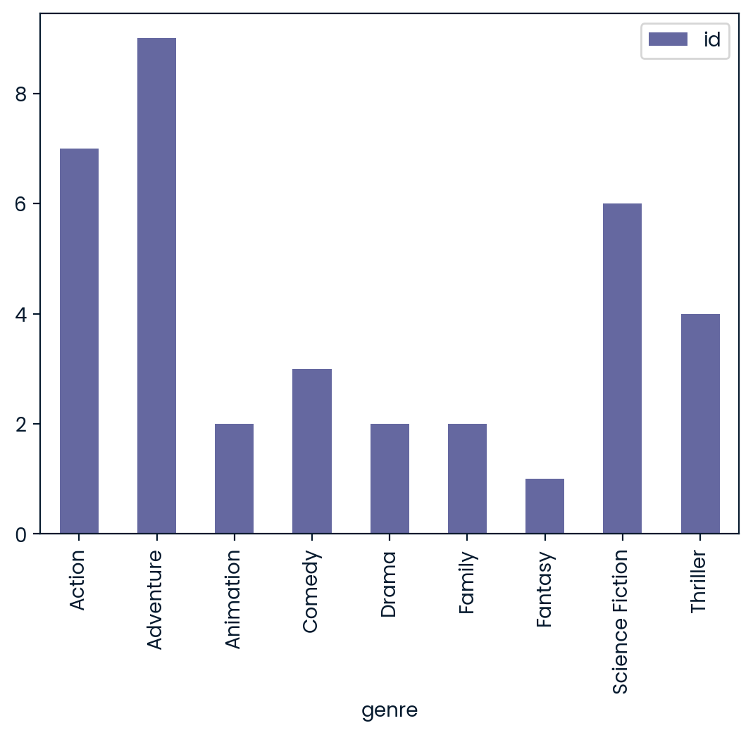
Using outer join to select actors
One cool aspect of using an outer join is that, because it returns all rows from both merged tables and null where they do not match, you can use it to find rows that do not have a match in the other table. To try for yourself, you have been given two tables with a list of actors from two popular movies: Iron Man 1 and Iron Man 2. Most of the actors played in both movies. Use an outer join to find actors who did not act in both movies.
The Iron Man 1 table is called iron_1_actors, and Iron Man 2 table is called iron_2_actors. Both tables have been loaded for you and a few rows printed so you can see the structure.
Instructions
- Save to iron_1_and_2 the merge of iron_1_actors (left) with iron_2_actors tables with an outer join on the id column, and set suffixes to (‘_1’,‘_2’).
- Create an index that returns True if name_1 or name_2 are null, and False otherwise.
casts = pd.read_pickle("datasets/casts.p")
casts.head(3)| movie_id | cast_id | character | gender | id | name | |
|---|---|---|---|---|---|---|
| 7 | 5 | 22 | Jezebel | 1 | 3122 | Sammi Davis |
| 8 | 5 | 23 | Diana | 1 | 3123 | Amanda de Cadenet |
| 9 | 5 | 24 | Athena | 1 | 3124 | Valeria Golino |
movies[movies.title.str.contains("Iron")]| id | title | popularity | release_date | |
|---|---|---|---|---|
| 181 | 10386 | The Iron Giant | 61.245957 | 1999-08-06 |
| 2198 | 1726 | Iron Man | 120.725053 | 2008-04-30 |
| 3041 | 38543 | Ironclad | 12.317080 | 2011-03-03 |
| 3271 | 97430 | The Man with the Iron Fists | 17.672021 | 2012-11-02 |
| 3286 | 68721 | Iron Man 3 | 77.682080 | 2013-04-18 |
| 3401 | 10138 | Iron Man 2 | 77.300194 | 2010-04-28 |
| 3900 | 9313 | The Man in the Iron Mask | 28.980270 | 1998-03-12 |
| 4539 | 71688 | The Iron Lady | 23.378400 | 2011-12-30 |
iron_1_actors = casts[casts.movie_id==1726]
iron_1_actors.head(3)| movie_id | cast_id | character | gender | id | name | |
|---|---|---|---|---|---|---|
| 3 | 1726 | 9 | Yinsen | 2 | 17857 | Shaun Toub |
| 4 | 1726 | 10 | Virginia “Pepper” Potts | 1 | 12052 | Gwyneth Paltrow |
| 2 | 1726 | 11 | Obadiah Stane / Iron Monger | 2 | 1229 | Jeff Bridges |
iron_2_actors = casts[casts.movie_id==10138]
iron_2_actors.head(3)| movie_id | cast_id | character | gender | id | name | |
|---|---|---|---|---|---|---|
| 4 | 10138 | 3 | Ivan Vanko / Whiplash | 2 | 2295 | Mickey Rourke |
| 3 | 10138 | 5 | Natalie Rushman / Natasha Romanoff / Black Widow | 1 | 1245 | Scarlett Johansson |
| 5 | 10138 | 6 | Justin Hammer | 2 | 6807 | Sam Rockwell |
# Merge iron_1_actors to iron_2_actors on id with outer join using suffixes
iron_1_and_2 = iron_1_actors.merge(iron_2_actors,
                                     on = "id",
                                     how='outer',
                                     suffixes=("_1","_2"))

# Create an index that returns true if name_1 or name_2 are null
m = ((iron_1_and_2['name_1'].isnull()) |
     (iron_1_and_2['name_2'].isnull()))

# Print the first few rows of iron_1_and_2
print(iron_1_and_2[m].head())
movie_id_1 cast_id_1 ... gender_2 name_2
0 1726.0 9.0 ... NaN NaN
2 1726.0 11.0 ... NaN NaN
3 1726.0 12.0 ... NaN NaN
5 1726.0 18.0 ... NaN NaN
8 1726.0 23.0 ... NaN NaN
[5 rows x 11 columns]Self join
Merging a table to itself can be useful when you want to compare values in a column to other values in the same column. In this exercise, you will practice this by creating a table that for each movie will list the movie director and a member of the crew on one row. You have been given a table called crews, which has columns id, job, and name. First, merge the table to itself using the movie ID. This merge will give you a larger table where for each movie, every job is matched against each other. Then select only those rows with a director in the left table, and avoid having a row where the director’s job is listed in both the left and right tables. This filtering will remove job combinations that aren’t with the director.
The crews table has been loaded for you. ### Instructions - To a variable called crews_self_merged, merge the crews table to itself on the id column using an inner join, setting the suffixes to ‘_dir’ and ‘_crew’ for the left and right tables respectively. - Create a Boolean index, named boolean_filter, that selects rows from the left table with the job of ‘Director’ and avoids rows with the job of ‘Director’ in the right table. - Use the .head() method to print the first few rows of direct_crews.
crews = pd.read_pickle("datasets/crews.p")
crews.head(3)| id | department | job | name | |
|---|---|---|---|---|
| 0 | 19995 | Editing | Editor | Stephen E. Rivkin |
| 2 | 19995 | Sound | Sound Designer | Christopher Boyes |
| 4 | 19995 | Production | Casting | Mali Finn |
# Merge the crews table to itself
crews_self_merged = crews.merge(crews,on = 'id',suffixes = ("_dir","_crew"))
# Merge the crews table to itself
crews_self_merged = crews.merge(crews, on='id', how='inner',
suffixes=('_dir','_crew'))
# Create a Boolean index to select the appropriate
boolean_filter = ((crews_self_merged['job_dir'] == "Director") &
(crews_self_merged['job_crew'] != "Director"))
direct_crews = crews_self_merged[boolean_filter]# Merge the crews table to itself
crews_self_merged = crews.merge(crews, on='id', how='inner',
suffixes=('_dir','_crew'))
# Create a boolean index to select the appropriate rows
boolean_filter = ((crews_self_merged['job_dir'] == 'Director') &
(crews_self_merged['job_crew'] != 'Director'))
direct_crews = crews_self_merged[boolean_filter]
# Print the first few rows of direct_crews
print(direct_crews.head()) id department_dir ... job_crew name_crew
156 19995 Directing ... Editor Stephen E. Rivkin
157 19995 Directing ... Sound Designer Christopher Boyes
158 19995 Directing ... Casting Mali Finn
160 19995 Directing ... Writer James Cameron
161 19995 Directing ... Set Designer Richard F. Mays
[5 rows x 7 columns]Index merge for movie ratings
To practice merging on indexes, you will merge movies and a table called ratings that holds info about movie ratings. Make sure your merge returns all of the rows from the movies table and not all the rows of ratings table need to be included in the result.
The movies and ratings tables have been loaded for you. ### Instructions - Merge movies and ratings on the index and save to a variable called movies_ratings, ensuring that all of the rows from the movies table are returned.
# Merge to the movies table the ratings table on the index
movies_ratings = movies.merge(ratings,on = 'id')

# Print the first few rows of movies_ratings
print(movies_ratings.head())
id title ... vote_average vote_count
0 257 Oliver Twist ... 6.7 274.0
1 14290 Better Luck Tomorrow ... 6.5 27.0
2 38365 Grown Ups ... 6.0 1705.0
3 9672 Infamous ... 6.4 60.0
4 12819 Alpha and Omega ... 5.3 124.0
[5 rows x 6 columns]Do sequels earn more?
It is time to put together many of the aspects that you have learned in this chapter. In this exercise, you’ll find out which movie sequels earned the most compared to the original movie. To answer this question, you will merge a modified version of the sequels and financials tables where their index is the movie ID. You will need to choose a merge type that will return all of the rows from the sequels table and not all the rows of financials table need to be included in the result. From there, you will join the resulting table to itself so that you can compare the revenue values of the original movie to the sequel. Next, you will calculate the difference between the two revenues and sort the resulting dataset.
The sequels and financials tables have been provided. ### Instructions - With the sequels table on the left, merge to it the financials table on index named id, ensuring that all the rows from the sequels are returned and some rows from the other table may not be returned, Save the results to sequels_fin. - Merge the sequels_fin table to itself with an inner join, where the left and right tables merge on sequel and id respectively with suffixes equal to (‘_org’,‘_seq’), saving to orig_seq. - Select the title_org, title_seq, and diff columns of orig_seq and save this as titles_diff. - Sort by titles_diff by diff in descending order and print the first few rows.
sequels = pd.read_pickle("datasets/sequels.p")
print(sequels.head(3))
financials = pd.read_pickle("datasets/financials.p")
print(financials.head(3))
id title sequel
0 19995 Avatar <NA>
1 862 Toy Story 863
2 863 Toy Story 2 10193
id budget revenue
0 19995 237000000 2.787965e+09
1 285 300000000 9.610000e+08
2 206647 245000000 8.806746e+08# Merge sequels and financials on index id
sequels_fin = sequels.merge(financials,on = 'id', how = "left")
sequels_fin.shape(4803, 5)# Merge sequels and financials on index id
sequels_fin = sequels.merge(financials, on='id', how='left')
sequels_fin.set_index("id", inplace=True)
# Self merge with suffixes as inner join with left on sequel and right on id
orig_seq = sequels_fin.merge(sequels_fin, left_on='sequel',
right_on='id', right_index=True,
suffixes=("_org","_seq"))
# Add calculation to subtract revenue_org from revenue_seq
orig_seq['diff'] = orig_seq['revenue_seq'] - orig_seq['revenue_org']# Merge sequels and financials on index id
sequels_fin = sequels.merge(financials, on='id', how='left')
sequels_fin.set_index("id", inplace=True)
# Self merge with suffixes as inner join with left on sequel and right on id
orig_seq = sequels_fin.merge(sequels_fin, how='inner', left_on='sequel',
right_on='id', right_index=True,
suffixes=('_org','_seq'))
# Add calculation to subtract revenue_org from revenue_seq
orig_seq['diff'] = orig_seq['revenue_seq'] - orig_seq['revenue_org']
# Select the title_org, title_seq, and diff
titles_diff = orig_seq[["title_org", "title_seq", "diff" ]]# Merge sequels and financials on index id
sequels_fin = sequels.merge(financials, on='id', how='left')
sequels_fin.set_index("id", inplace=True)
# Self merge with suffixes as inner join with left on sequel and right on id
orig_seq = sequels_fin.merge(sequels_fin, how='inner', left_on='sequel',
right_on='id', right_index=True,
suffixes=('_org','_seq'))
# Add calculation to subtract revenue_org from revenue_seq
orig_seq['diff'] = orig_seq['revenue_seq'] - orig_seq['revenue_org']
# Select the title_org, title_seq, and diff
titles_diff = orig_seq[['title_org','title_seq','diff']]
# Print the first rows of the sorted titles_diff
print(titles_diff.sort_values("diff", ascending=False).head()) title_org title_seq diff
id
331 Jurassic Park III Jurassic World 1.144748e+09
272 Batman Begins The Dark Knight 6.303398e+08
10138 Iron Man 2 Iron Man 3 5.915067e+08
863 Toy Story 2 Toy Story 3 5.696028e+08
10764 Quantum of Solace Skyfall 5.224703e+08Chapter 3: Advanced Merging and Concatenating
In this chapter, you’ll leverage powerful filtering techniques, including semi-joins and anti-joins. You’ll also learn how to glue DataFrames by vertically combining and using the pandas.concat function to create new datasets. Finally, because data is rarely clean, you’ll also learn how to validate your newly combined data structures.
Performing an anti join
In our music streaming company dataset, each customer is assigned an employee representative to assist them. In this exercise, filter the employee table by a table of top customers, returning only those employees who are not assigned to a customer. The results should resemble the results of an anti join. The company’s leadership will assign these employees additional training so that they can work with high valued customers.
The top_cust and employees tables have been provided for you. ### Instructions - Merge employees and top_cust with a left join, setting indicator argument to True. Save the result to empl_cust. - Select the srid column of empl_cust and the rows where _merge is ‘left_only’. Save the result to srid_list. - Subset the employees table and select those rows where the srid is in the variable srid_list and print the results.
employees = pd.read_csv("datasets/employee.csv")
employees.head(2)| ind | srid | lname | fname | title | hire_date | ||
|---|---|---|---|---|---|---|---|
| 0 | 0 | 1 | Adams | Andrew | General Manager | 2002-08-14 | andrew@chinookcorp.com |
| 1 | 1 | 2 | Edwards | Nancy | Sales Manager | 2002-05-01 | nancy@chinookcorp.com |
top_cust = pd.read_csv("datasets/top_cust.csv")
top_cust.columns
Index(['cid', 'srid', 'fname', 'lname', 'phone', 'fax', 'email'], dtype='object')# Merge employees and top_cust
empl_cust = employees.merge(top_cust, on='srid',
how="left", indicator=True)# Merge employees and top_cust
empl_cust = employees.merge(top_cust, on='srid',
how='left', indicator=True)
# Select the srid column where _merge is left_only
srid_list = empl_cust.loc[empl_cust["_merge"]=='left_only', 'srid']# Merge employees and top_cust
empl_cust = employees.merge(top_cust, on='srid',
how='left', indicator=True)
# Select the srid column where _merge is left_only
srid_list = empl_cust.loc[empl_cust['_merge'] == 'left_only', 'srid']
# Get employees not working with top customers
print(employees[employees.srid.isin(srid_list)]) ind srid ... hire_date email
0 0 1 ... 2002-08-14 andrew@chinookcorp.com
1 1 2 ... 2002-05-01 nancy@chinookcorp.com
5 5 6 ... 2003-10-17 michael@chinookcorp.com
6 6 7 ... 2004-01-02 robert@chinookcorp.com
7 7 8 ... 4/3/2004 laura@chinookcorp.com
[5 rows x 7 columns]Performing a semi join
Some of the tracks that have generated the most significant amount of revenue are from TV-shows or are other non-musical audio. You have been given a table of invoices that include top revenue-generating items. Additionally, you have a table of non-musical tracks from the streaming service. In this exercise, you’ll use a semi join to find the top revenue-generating non-musical tracks..
The tables non_mus_tcks, top_invoices, and genres have been loaded for you.
Instructions
- Merge non_mus_tcks and top_invoices on tid using an inner join. Save the result as tracks_invoices.
- Use .isin() to subset the rows of non_mus_tck where tid is in the tid column of tracks_invoices. Save the result as top_tracks.
- Group top_tracks by gid and count the tid rows. Save the result to cnt_by_gid.
- Merge cnt_by_gid with the genres table on gid and print the result.
# Merge the non_mus_tck and top_invoices tables on tid
tracks_invoices = non_mus_tcks.merge(top_invoices,on = 'tid')

# Use .isin() to subset non_mus_tcks to rows with tid in tracks_invoices
top_tracks = non_mus_tcks[non_mus_tcks['tid'].isin(tracks_invoices.tid)]

# Group the top_tracks by gid and count the tid rows
cnt_by_gid = top_tracks.groupby(['gid'], as_index=False).agg({'tid':'count'})

# Merge the genres table to cnt_by_gid on gid and print
print(cnt_by_gid.merge(genres, on ="gid"))
Concatenation basics
You have been given a few tables of data with musical track info for different albums from the metal band, Metallica. The track info comes from their Ride The Lightning, Master Of Puppets, and St. Anger albums. Try various features of the .concat() method by concatenating the tables vertically together in different ways.
The tables tracks_master, tracks_ride, and tracks_st have loaded for you. ### Instructions - Concatenate tracks_master, tracks_ride, and tracks_st, in that order, setting sort to True. - Concatenate tracks_master, tracks_ride, and tracks_st, where the index goes from 0 to n-1. - Concatenate tracks_master, tracks_ride, and tracks_st, showing only columns that are in all tables.
# Concatenate the tracks
tracks_from_albums = pd.concat([tracks_master, tracks_ride, tracks_st],
                               sort=True)
print(tracks_from_albums)
# Concatenate the tracks so the index goes from 0 to n-1
tracks_from_albums = pd.concat([tracks_master, tracks_ride, tracks_st],
ignore_index = True,
sort=True)
print(tracks_from_albums)# Concatenate the tracks, show only columns names that are in all tables
tracks_from_albums = pd.concat([tracks_master, tracks_ride,tracks_st],
join = 'inner',
sort=True)
print(tracks_from_albums)Concatenating with keys
The leadership of the music streaming company has come to you and asked you for assistance in analyzing sales for a recent business quarter. They would like to know which month in the quarter saw the highest average invoice total. You have been given three tables with invoice data named inv_jul, inv_aug, and inv_sep. Concatenate these tables into one to create a graph of the average monthly invoice total.
Instructions
- Concatenate the three tables together vertically in order with the oldest month first, adding ‘7Jul’, ‘8Aug’, and ‘9Sep’ as keys for their respective months, and save to variable avg_inv_by_month.
- Use the .agg() method to find the average of the total column from the grouped invoices.
- Create a bar chart of avg_inv_by_month.
# Concatenate the tables and add keys
inv_jul_thr_sep = pd.concat([inv_jul, inv_aug, inv_sep],
                            keys=['7Jul', '8Aug', '9Sep'])

# Group the invoices by the index keys and find avg of the total column
avg_inv_by_month = inv_jul_thr_sep.groupby(level=0).agg({"total":"mean"})

# Bar plot of avg_inv_by_month
avg_inv_by_month.plot(kind="bar")
plt.show()
Concatenate and merge to find common songs
The senior leadership of the streaming service is requesting your help again. You are given the historical files for a popular playlist in the classical music genre in 2018 and 2019. Additionally, you are given a similar set of files for the most popular pop music genre playlist on the streaming service in 2018 and 2019. Your goal is to concatenate the respective files to make a large classical playlist table and overall popular music table. Then filter the classical music table using a semi join to return only the most popular classical music tracks.
The tables classic_18, classic_19, and pop_18, pop_19 have been loaded for you. Additionally, pandas has been loaded as pd. ### Instructions - Concatenate the classic_18 and classic_19 tables vertically where the index goes from 0 to n-1, and save to classic_18_19. - Concatenate the pop_18 and pop_19 tables vertically where the index goes from 0 to n-1, and save to pop_18_19. - With classic_18_19 on the left, merge it with pop_18_19 on tid using an inner join. - Use .isin() to filter classic_18_19 where tid is in classic_pop.
# Concatenate the classic tables vertically
classic_18_19 = pd.concat([classic_18, classic_19],ignore_index=True)

# Concatenate the pop tables vertically
pop_18_19 = pd.concat([pop_18, pop_19], ignore_index = True)- With classic_18_19 on the left, merge it with pop_18_19 on tid using an inner join.
- Use .isin() to filter classic_18_19 where tid is in classic_pop.
# Concatenate the classic tables vertically
classic_18_19 = pd.concat([classic_18, classic_19], ignore_index=True)

# Concatenate the pop tables vertically
pop_18_19 = pd.concat([pop_18, pop_19], ignore_index=True)

# Merge classic_18_19 with pop_18_19
classic_pop = classic_18_19.merge(pop_18_19,on='tid')

# Using .isin(), filter classic_18_19 rows where tid is in classic_pop
popular_classic = classic_18_19[classic_18_19["tid"].isin(classic_pop.tid)]

# Print popular chart
print(popular_classic)
Chapter 4: Merging Ordered and Time-Series Data
In this final chapter, you’ll step up a gear and learn to apply pandas’ specialized methods for merging time-series and ordered data together with real-world financial and economic data from the city of Chicago. You’ll also learn how to query resulting tables using a SQL-style format, and unpivot data using the melt method.
Correlation between GDP and S&P500
In this exercise, you want to analyze stock returns from the S&P 500. You believe there may be a relationship between the returns of the S&P 500 and the GDP of the US. Merge the different datasets together to compute the correlation.
Two tables have been provided for you, named sp500, and gdp. As always, pandas has been imported for you as pd. Instructions - Use merge_ordered() to merge gdp and sp500 using a left join on year and date. Save the results as gdp_sp500. - Print gdp_sp500 and look at the returns for the year 2018.
gdp = pd.read_csv("datasets/WorldBank_GDP.csv")
print(gdp.head(4))
sp500 = pd.read_csv("datasets/S&P500.csv")
sp500.head(3)
Country Name Country Code Indicator Name Year GDP
0 China CHN GDP (current US$) 2010 6.087160e+12
1 Germany DEU GDP (current US$) 2010 3.417090e+12
2 Japan JPN GDP (current US$) 2010 5.700100e+12
3 United States USA GDP (current US$) 2010 1.499210e+13| Date | Returns | |
|---|---|---|
| 0 | 2008 | -38.49 |
| 1 | 2009 | 23.45 |
| 2 | 2010 | 12.78 |
# Use merge_ordered() to merge gdp and sp500 on year and date
gdp_sp500 = pd.merge_ordered(gdp, sp500, left_on='Year', right_on='Date',
                             how='left')

# Print gdp_sp500
print(gdp_sp500)
Country Name Country Code ... Date Returns
0 China CHN ... 2010.0 12.78
1 Germany DEU ... 2010.0 12.78
2 Japan JPN ... 2010.0 12.78
3 United States USA ... 2010.0 12.78
4 China CHN ... 2011.0 0.00
5 Germany DEU ... 2011.0 0.00
6 Japan JPN ... 2011.0 0.00
7 United States USA ... 2011.0 0.00
8 China CHN ... 2012.0 13.41
9 Germany DEU ... 2012.0 13.41
10 Japan JPN ... 2012.0 13.41
11 United States USA ... 2012.0 13.41
12 China CHN ... 2012.0 13.41
13 Germany DEU ... 2012.0 13.41
14 Japan JPN ... 2012.0 13.41
15 United States USA ... 2012.0 13.41
16 China CHN ... 2013.0 29.60
17 Germany DEU ... 2013.0 29.60
18 Japan JPN ... 2013.0 29.60
19 United States USA ... 2013.0 29.60
20 China CHN ... 2014.0 11.39
21 Germany DEU ... 2014.0 11.39
22 Japan JPN ... 2014.0 11.39
23 United States USA ... 2014.0 11.39
24 China CHN ... 2015.0 -0.73
25 Germany DEU ... 2015.0 -0.73
26 Japan JPN ... 2015.0 -0.73
27 United States USA ... 2015.0 -0.73
28 China CHN ... 2016.0 9.54
29 Germany DEU ... 2016.0 9.54
30 Japan JPN ... 2016.0 9.54
31 United States USA ... 2016.0 9.54
32 China CHN ... 2017.0 19.42
33 Germany DEU ... 2017.0 19.42
34 Japan JPN ... 2017.0 19.42
35 United States USA ... 2017.0 19.42
36 China CHN ... NaN NaN
37 Germany DEU ... NaN NaN
38 Japan JPN ... NaN NaN
39 United States USA ... NaN NaN
[40 rows x 7 columns]- Use merge_ordered(), again similar to before, to merge gdp and sp500 use the function’s ability to interpolate missing data to forward fill the missing value for returns, assigning this table to the variable gdp_sp500.
# Use merge_ordered() to merge gdp and sp500, interpolate missing value
gdp_sp500 = pd.merge_ordered(gdp, sp500,left_on='Year',right_on='Date',how="left",fill_method='ffill')


# Print gdp_sp500
print (gdp_sp500)
Country Name Country Code Indicator Name ... GDP Date Returns
0 China CHN GDP (current US$) ... 6.087160e+12 2010 12.78
1 Germany DEU GDP (current US$) ... 3.417090e+12 2010 12.78
2 Japan JPN GDP (current US$) ... 5.700100e+12 2010 12.78
3 United States USA GDP (current US$) ... 1.499210e+13 2010 12.78
4 China CHN GDP (current US$) ... 7.551500e+12 2011 0.00
5 Germany DEU GDP (current US$) ... 3.757700e+12 2011 0.00
6 Japan JPN GDP (current US$) ... 6.157460e+12 2011 0.00
7 United States USA GDP (current US$) ... 1.554260e+13 2011 0.00
8 China CHN GDP (current US$) ... 8.532230e+12 2012 13.41
9 Germany DEU GDP (current US$) ... 3.543980e+12 2012 13.41
10 Japan JPN GDP (current US$) ... 6.203210e+12 2012 13.41
11 United States USA GDP (current US$) ... 1.619700e+13 2012 13.41
12 China CHN GDP (current US$) ... 8.532230e+12 2012 13.41
13 Germany DEU GDP (current US$) ... 3.543980e+12 2012 13.41
14 Japan JPN GDP (current US$) ... 6.203210e+12 2012 13.41
15 United States USA GDP (current US$) ... 1.619700e+13 2012 13.41
16 China CHN GDP (current US$) ... 9.570410e+12 2013 29.60
17 Germany DEU GDP (current US$) ... 3.752510e+12 2013 29.60
18 Japan JPN GDP (current US$) ... 5.155720e+12 2013 29.60
19 United States USA GDP (current US$) ... 1.678480e+13 2013 29.60
20 China CHN GDP (current US$) ... 1.043850e+13 2014 11.39
21 Germany DEU GDP (current US$) ... 3.898730e+12 2014 11.39
22 Japan JPN GDP (current US$) ... 4.850410e+12 2014 11.39
23 United States USA GDP (current US$) ... 1.752170e+13 2014 11.39
24 China CHN GDP (current US$) ... 1.101550e+13 2015 -0.73
25 Germany DEU GDP (current US$) ... 3.381390e+12 2015 -0.73
26 Japan JPN GDP (current US$) ... 4.389480e+12 2015 -0.73
27 United States USA GDP (current US$) ... 1.821930e+13 2015 -0.73
28 China CHN GDP (current US$) ... 1.113790e+13 2016 9.54
29 Germany DEU GDP (current US$) ... 3.495160e+12 2016 9.54
30 Japan JPN GDP (current US$) ... 4.926670e+12 2016 9.54
31 United States USA GDP (current US$) ... 1.870720e+13 2016 9.54
32 China CHN GDP (current US$) ... 1.214350e+13 2017 19.42
33 Germany DEU GDP (current US$) ... 3.693200e+12 2017 19.42
34 Japan JPN GDP (current US$) ... 4.859950e+12 2017 19.42
35 United States USA GDP (current US$) ... 1.948540e+13 2017 19.42
36 China CHN GDP (current US$) ... 1.360820e+13 2017 19.42
37 Germany DEU GDP (current US$) ... 3.996760e+12 2017 19.42
38 Japan JPN GDP (current US$) ... 4.970920e+12 2017 19.42
39 United States USA GDP (current US$) ... 2.049410e+13 2017 19.42
[40 rows x 7 columns]- Subset the gdp_sp500 table, select the gdp and returns columns, and save as gdp_returns.
- Print the correlation matrix of the gdp_returns table using the .corr() method.
# Use merge_ordered() to merge gdp and sp500, interpolate missing value
gdp_sp500 = pd.merge_ordered(gdp, sp500, left_on='Year', right_on='Date',
                             how='left',  fill_method='ffill')

# Subset the gdp and returns columns
gdp_returns = gdp_sp500[["GDP","Returns"]]

# Print gdp_returns correlation
print (gdp_returns.corr())
GDP Returns
GDP 1.000000 0.040669
Returns 0.040669 1.000000Phillips curve using merge_ordered()
There is an economic theory developed by A. W. Phillips which states that inflation and unemployment have an inverse relationship. The theory claims that with economic growth comes inflation, which in turn should lead to more jobs and less unemployment.
You will take two tables of data from the U.S. Bureau of Labor Statistics, containing unemployment and inflation data over different periods, and create a Phillips curve. The tables have different frequencies. One table has a data entry every six months, while the other has a data entry every month. You will need to use the entries where you have data within both tables.
The tables unemployment and inflation have been loaded for you. ### Instructions - Use merge_ordered() to merge the inflation and unemployment tables on date with an inner join, and save the results as inflation_unemploy. - Print the inflation_unemploy variable. - Using inflation_unemploy, create a scatter plot with unemployment_rate on the horizontal axis and cpi (inflation) on the vertical axis.
# Use merge_ordered() to merge inflation, unemployment with inner join
inflation_unemploy = pd.merge_ordered(inflation, unemployment, how="inner", on = "date")

# Print inflation_unemploy
print(inflation_unemploy)

# Plot a scatter plot of unemployment_rate vs cpi of inflation_unemploy
inflation_unemploy.plot(x="unemployment_rate", y = "cpi", kind='scatter')
plt.show()
merge_ordered() caution, multiple columns
When using merge_ordered() to merge on multiple columns, the order is important when you combine it with the forward fill feature. The function sorts the merge on columns in the order provided. In this exercise, we will merge GDP and population data from the World Bank for the Australia and Sweden, reversing the order of the merge on columns. The frequency of the series are different, the GDP values are quarterly, and the population is yearly. Use the forward fill feature to fill in the missing data. Depending on the order provided, the fill forward will use unintended data to fill in the missing values.
The tables gdp and pop have been loaded. ### Instructions - Use merge_ordered() on gdp and pop, merging on columns date and country with the fill feature, save to ctry_date. - Perform the same merge of gdp and pop, but join on country and date (reverse of step 1) with the fill feature, saving this as date_ctry.
pop = pd.read_csv("datasets/WorldBank_POP.csv")
pop.head(3)| Country Name | Country Code | Indicator Name | Year | Pop | |
|---|---|---|---|---|---|
| 0 | Aruba | ABW | Population, total | 2010 | 101669.0 |
| 1 | Afghanistan | AFG | Population, total | 2010 | 29185507.0 |
| 2 | Angola | AGO | Population, total | 2010 | 23356246.0 |
# Merge gdp and pop on date and country with fill and notice rows 2 and 3
ctry_date = pd.merge_ordered(gdp,pop,on=['Year','Country Name'],
                             fill_method='ffill')

# Print ctry_date
print(ctry_date)
Country Name Country Code_x ... Indicator Name_y Pop
0 Afghanistan NaN ... Population, total 2.918551e+07
1 Albania NaN ... Population, total 2.913021e+06
2 Algeria NaN ... Population, total 3.597746e+07
3 American Samoa NaN ... Population, total 5.607900e+04
4 Andorra NaN ... Population, total 8.444900e+04
... ... ... ... ... ...
2643 West Bank and Gaza USA ... Population, total 4.569087e+06
2644 World USA ... Population, total 7.594270e+09
2645 Yemen, Rep. USA ... Population, total 2.849869e+07
2646 Zambia USA ... Population, total 1.735182e+07
2647 Zimbabwe USA ... Population, total 1.443902e+07
[2648 rows x 8 columns]# Merge gdp and pop on country and date with fill
date_ctry = pd.merge_ordered(gdp,pop,on = ["Country Name","Year"],fill_method='ffill')
# Print date_ctry
print(date_ctry) Country Name Country Code_x ... Indicator Name_y Pop
0 Afghanistan NaN ... Population, total 29185507.0
1 Afghanistan NaN ... Population, total 30117413.0
2 Afghanistan NaN ... Population, total 31161376.0
3 Afghanistan NaN ... Population, total 31161376.0
4 Afghanistan NaN ... Population, total 32269589.0
... ... ... ... ... ...
2643 Zimbabwe USA ... Population, total 13586681.0
2644 Zimbabwe USA ... Population, total 13814629.0
2645 Zimbabwe USA ... Population, total 14030390.0
2646 Zimbabwe USA ... Population, total 14236745.0
2647 Zimbabwe USA ... Population, total 14439018.0
[2648 rows x 8 columns]Using merge_asof() to study stocks
You have a feed of stock market prices that you record. You attempt to track the price every five minutes. Still, due to some network latency, the prices you record are roughly every 5 minutes. You pull your price logs for three banks, JP Morgan (JPM), Wells Fargo (WFC), and Bank Of America (BAC). You want to know how the price change of the two other banks compare to JP Morgan. Therefore, you will need to merge these three logs into one table. Afterward, you will use the pandas .diff() method to compute the price change over time. Finally, plot the price changes so you can review your analysis.
The three log files have been loaded for you as tables named jpm, wells, and bac. ## Instructions - Use merge_asof() to merge jpm (left table) and wells together on the date_time column, where the rows with the nearest times are matched, and with suffixes=(’‘,’_wells’). Save to jpm_wells. - Use merge_asof() to merge jpm_wells (left table) and bac together on the date_time column, where the rows with the closest times are matched, and with suffixes=(‘_jpm’, ‘_bac’). Save to jpm_wells_bac. - Using price_diffs, create a line plot of the close price of JPM, WFC, and BAC only.
# Use merge_asof() to merge jpm and wells
jpm_wells = pd.merge_asof(jpm, wells, on='date_time',
                          suffixes=('', '_wells'), direction='nearest')

# Use merge_asof() to merge jpm_wells and bac
jpm_wells_bac = pd.merge_asof(jpm_wells, bac, on='date_time',
                              suffixes=('_jpm', '_bac'), direction='nearest')

# Compute price diff
price_diffs = jpm_wells_bac.diff()

# Plot the price diff of the close of jpm, wells and bac only
price_diffs.plot(y=['close_jpm','close_wells','close_bac'])
plt.show()
Using merge_asof() to create dataset
The merge_asof() function can be used to create datasets where you have a table of start and stop dates, and you want to use them to create a flag in another table. You have been given gdp, which is a table of quarterly GDP values of the US during the 1980s. Additionally, the table recession has been given to you. It holds the starting date of every US recession since 1980, and the date when the recession was declared to be over. Use merge_asof() to merge the tables and create a status flag if a quarter was during a recession. Finally, to check your work, plot the data in a bar chart.
The tables gdp and recession have been loaded for you. ### Instructions - Using merge_asof(), merge gdp and recession on date, with gdp as the left table. Save to the variable gdp_recession. - Create a list using a list comprehension and a conditional expression, named is_recession, where for each row if the gdp_recession[‘econ_status’] value is equal to ‘recession’ then enter ‘r’ else ‘g’. - Using gdp_recession, plot a bar chart of gdp versus date, setting the color argument equal to is_recession.
# Merge gdp and recession on date using merge_asof()
gdp_recession = pd.merge_asof(gdp, recession, on='date')

# Create a list based on the row value of gdp_recession['econ_status']
is_recession = ['r' if s=='recession' else 'g' for s in gdp_recession['econ_status']]

# Plot a bar chart of gdp_recession
gdp_recession.plot(kind='bar', y='gdp', x='date', color=is_recession, rot=90)
plt.show()
Subsetting rows with .query()
In this exercise, you will revisit GDP and population data for Australia and Sweden from the World Bank and expand on it using the .query() method. You’ll merge the two tables and compute the GDP per capita. Afterwards, you’ll use the .query() method to sub-select the rows and create a plot. Recall that you will need to merge on multiple columns in the proper order.
The tables gdp and pop have been loaded for you. ### Instructions - Use merge_ordered() on gdp and pop on columns country and date with the fill feature, save to gdp_pop and print. - Add a column named gdp_per_capita to gdp_pop that divides gdp by pop. - Pivot gdp_pop so values=‘gdp_per_capita’, index=‘date’, and columns=‘country’, save as gdp_pivot. - Use .query() to select rows from gdp_pivot where date is greater than equal to “1991-01-01”. Save as recent_gdp_pop.
# Merge gdp and pop on date and country with fill
gdp_pop = pd.merge_ordered(gdp, pop, on=['country','date'], fill_method='ffill')
# Merge gdp and pop on date and country with fill
gdp_pop = pd.merge_ordered(gdp, pop, on=['country','date'], fill_method='ffill')
# Add a column named gdp_per_capita to gdp_pop that divides the gdp by pop
gdp_pop['gdp_per_capita'] = gdp_pop['gdp'] / gdp_pop['pop']# Merge gdp and pop on date and country with fill
gdp_pop = pd.merge_ordered(gdp, pop, on=['country','date'], fill_method='ffill')
# Add a column named gdp_per_capita to gdp_pop that divides the gdp by pop
gdp_pop['gdp_per_capita'] = gdp_pop['gdp'] / gdp_pop['pop']
# Pivot table of gdp_per_capita, where index is date and columns is country
gdp_pivot = gdp_pop.pivot_table('gdp_per_capita', 'date', 'country')# Merge gdp and pop on date and country with fill
gdp_pop = pd.merge_ordered(gdp, pop, on=['country','date'], fill_method='ffill')
# Add a column named gdp_per_capita to gdp_pop that divides the gdp by pop
gdp_pop['gdp_per_capita'] = gdp_pop['gdp'] / gdp_pop['pop']
# Pivot data so gdp_per_capita, where index is date and columns is country
gdp_pivot = gdp_pop.pivot_table('gdp_per_capita', 'date', 'country')
# Select dates equal to or greater than 1991-01-01
recent_gdp_pop = gdp_pivot.query('date >= "1991-01-01"')
# Plot recent_gdp_pop
recent_gdp_pop.plot(rot=90)
plt.show()Using .melt() to reshape government data
The US Bureau of Labor Statistics (BLS) often provides data series in an easy-to-read format - it has a separate column for each month, and each year is a different row. Unfortunately, this wide format makes it difficult to plot this information over time. In this exercise, you will reshape a table of US unemployment rate data from the BLS into a form you can plot using .melt(). You will need to add a date column to the table and sort by it to plot the data correctly.
The unemployment rate data has been loaded for you in a table called ur_wide. You are encouraged to explore this table before beginning the exercise. ### Instructions - Use .melt() to unpivot all of the columns of ur_wide except year and ensure that the columns with the months and values are named month and unempl_rate, respectively. Save the result as ur_tall. - Add a column to ur_tall named date which combines the year and month columns as year-month format into a larger string, and converts it to a date data type. - Sort ur_tall by date and save as ur_sorted. - Using ur_sorted, plot unempl_rate on the y-axis and date on the x-axis.
# Unpivot everything besides the year column
ur_tall = ur_wide.melt(id_vars=['year'], var_name='month',
                       value_name='unempl_rate')

# Create a date column using the month and year columns of ur_tall
ur_tall['date'] = pd.to_datetime(ur_tall['month'] + '-' + ur_tall['year'])

# Sort ur_tall by date in ascending order
ur_sorted = ur_tall.sort_values('date')

# Plot the unempl_rate by date
ur_sorted.plot(x='date', y='unempl_rate')
plt.show()
Using .melt() for stocks vs bond performance
It is widespread knowledge that the price of bonds is inversely related to the price of stocks. In this last exercise, you’ll review many of the topics in this chapter to confirm this. You have been given a table of percent change of the US 10-year treasury bond price. It is in a wide format where there is a separate column for each year. You will need to use the .melt() method to reshape this table.
Additionally, you will use the .query() method to filter out unneeded data. You will merge this table with a table of the percent change of the Dow Jones Industrial stock index price. Finally, you will plot data.
The tables ten_yr and dji have been loaded for you. ### Instructions - Use .melt() on ten_yr to unpivot everything except the metric column, setting var_name=‘date’ and value_name=‘close’. Save the result to bond_perc. - Using the .query() method, select only those rows were metric equals ‘close’, and save to bond_perc_close. - Use merge_ordered() to merge dji (left table) and bond_perc_close on date with an inner join, and set suffixes equal to (‘_dow’, ‘_bond’). Save the result to dow_bond. - Using dow_bond, plot only the Dow and bond values.
# Use melt on ten_yr, unpivot everything besides the metric column
bond_perc = ten_yr.melt(id_vars='metric', var_name='date', value_name='close')

# Use query on bond_perc to select only the rows where metric=close
bond_perc_close = bond_perc.query('metric == "close"')

# Merge (ordered) dji and bond_perc_close on date with an inner join
dow_bond = pd.merge_ordered(dji, bond_perc_close, on='date',
                            suffixes=('_dow', '_bond'), how='inner')

# Plot only the close_dow and close_bond columns
dow_bond.plot(y=['close_dow', 'close_bond'], x='date', rot=90)
plt.show()